Excel Dependent Drop Down List Example

This article will tell you how to create an excel dependent drop-down list with examples.

1. How To Create Excel Dependent Drop Down List Example.

1.1 Excel Dependent Drop-Down List Example Introduction.

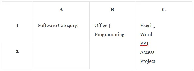
1. There are 2 list cells in this example.
2. The first list in cell B1 contains 2 items which are Office and Programming.
3. When you select the item Office from the first list, then it will show a list containing 5 items which are Excel, Word, PPT, Access, and Project in the second list in cell C1.
4. When you select the item Programming from the first list in cell B1, then it will show a list containing 3 items which are Visual Studio Code, Eclipse, and PyCharm in the second list in cell C1.
5. So the second drop-down list cell’s data will depend on the first drop-down list cell’s data change.
6. Below are the example worksheet cells.
   

1.2 How To Create Excel Dependent Drop-Down List.

1.2.1 Create The First Named Range With The Name Software.

1. Input the below data in cells E1 and E2.
   
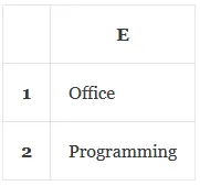
2. Select cells E1 and E2, then click the Formulas tab —> Define Name item in the Defined Names group.
3. Input the text Software in the Name input text box, then click the OK button to create the first named range, the range object’s name is Software.

1.2.2 Create The Second Named Range With The Name Office.

1. Input the below cell data in the cell range F1:F5.
   
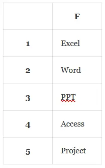
2. Select the cell range F1:F5 and create the second named range with the name Office.
3. The name Office is the first item value of the named range Software.

1.2.3 Create The Third Named Range With The Name Programming.

1. Input the below cell data in the cell range G1:G3.
   
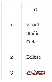
2. Select the cell range G1:G3, and create the third named range with the name Programming.
3. The name Programming is the second item value of the named range Software.

1.2.4 Create The Dependent Drop-Down List.

1. Click to select cell B1, then click the Data tab —> Data Validation item in the Data Tools group to open the Data Validation dialog.
2. Select the item List from the Allow drop-down list in the Settings tab.
3. Input the formula =Software in the Source text box, then it will show the data of the named range Software in the cell.
4. Click the OK button to save and exit the dialog.
5. Select cell C1 and open the Data Validation dialog window like above.
6. Select the item List from the Allow drop-down list in the Settings tab.
7. Input the formula =INDIRECT($B$1) in the Source input text box.
8. The formula uses the excel INDIRECT function to convert the text to a valid excel reference.
9. Then =INDIRECT(“Office”) will return the named range Office, and =INDIRECT(“Programming”) will return the named range Programming.
10. So that when you select a different item in the cell B1 list, cell C1 will display different list data accordingly.

References

1. How To Define Named Constant In Excel And Create Excel Named Range.
2. How To Use Excel Indirect Function Examples.