Excel Find First / Last Non-Empty Cell In Row / Column Example

In this article, I will tell you how to use the excel INDEX & MATCH function to find the first non-empty cell in a row or column, it will also tell you how to use the excel LOOKUP function to find the last non-empty cell in a row or column with examples.

Table of Contents

1. How To Use Excel INDEX & MATCH Function To Find The First Non-Empty Cell In A Row Or Column.

Below is cthis article’s example’s source cell data.
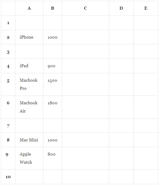
If you want to get the first non-empty cell in column A, you can use the below formula.
```
=INDEX(A1:A10,MATCH(TRUE,INDEX((A1:A10<>0),0),0))
```
Input the above formula into cell C1 and press the enter key, then it will show the text iPhone in cell C1.
Because the text iPhone is the first non-empty cell’s text in column A.
The formula uses both excel INDEX and MATCH functions, now I will explain the formula to you.

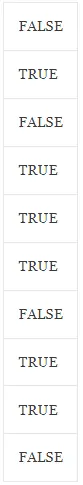
1.1 (A1:A10<>0).

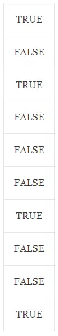
The (A1:A10<>0) part in the formula will return a boolean list, and each element in the list will be TRUE or FALSE
It will compare each cell value in the cell range A1:A10 to the value 0, if the cell value is not 0 ( or not empty ) then return TRUE, if the cell value is 0 ( or empty ) then return FALSE.
If you input the formula =(A1:A10<>0) in cell C1 and press the enter key, then you can get the below column in cell range C1:C10.

1.2 INDEX((A1:A10<>0),0).

The excel INDEX function is used to find and return the value in a specified cell range located by provided row and column number. You can read the article How To Use Excel Index Function With Examples to learn how to use it.
So the INDEX((A1:A10<>0),0) part will return the first column in the boolean list generated by the (A1:A10<>0) part.
So when you input the formula =INDEX((A1:A10<>0),0) in cell C1, it will show the below boolean column in cell range C1:C10 also.

1.3 MATCH(TRUE,INDEX((A1:A10<>0),0),0).

The excel MATCH function will return the first element’s position number that matches the search value in the value list, you can read the article How To Use Excel Match Function With Examples to learn more.
In this formula, it will find the first cell’s position number that value is TRUE in the value list generated by the formula INDEX((A1:A10<>0),0).
Input the formula =MATCH(TRUE, INDEX((A1:A10<>0),0),0) in cell C1 and press the enter key, then it will show the number 2 in cell C1.
Passing 0 to the third argument of the MATCH function means an exact match.
And because the second cell’s ( cell A2 ) value is not empty, then it returns the cell A2‘s position number which is number 2.

1.4 INDEX(A1:A10,MATCH(TRUE,INDEX((A1:A10<>0),0),0),1).

This formula =INDEX(A1:A10, MATCH(TRUE, INDEX((A1:A10<>0),0),0),1) can be translated to =INDEX(A1:A10,2,1) then it will return the second cell ( cell A2 ) ‘s value ( iPhone ) in the cell.

2. How To Use Excel LOOKUP Function To Find The Last Non-Empty Cell In A Row Or Column.

Now we will use the excel LOOKUP function to find the last non-empty cell in a row or column.
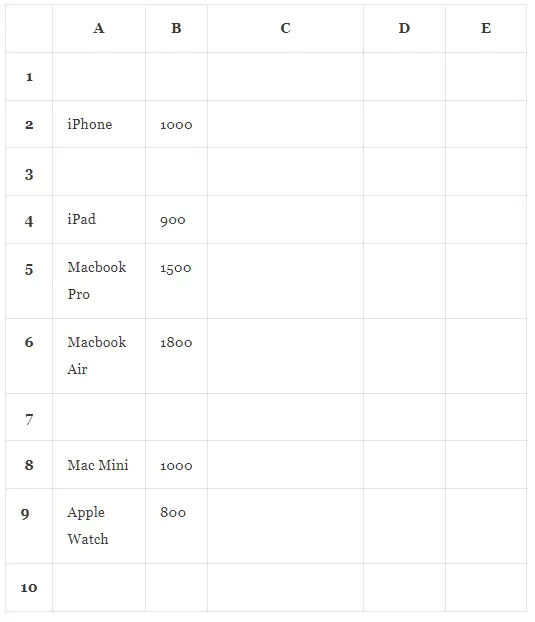
We still use the above example data cells.
Input the formula =LOOKUP(2,1/(NOT(ISBLANK(A1:A10))), A1:A10) in cell C1 and press the enter key, then it will show the text Apple Watch ( the last non-empty cell A9‘s value ) in cell C1.
Now I will explain the formula to you part by part.
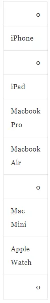
Input the formula =A1:A10 in cell C1 then it will display the value list as below.
Input the formula =ISBLANK(A1:A10) in cell C1 then it will show the below value list.
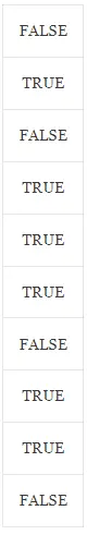
And the formula =NOT(ISBLANK(A1:A10)) will return the below value list.
The formula =1/(NOT(ISBLANK(A1:A10))) will return the below value list. If the cell value is empty then the formula 1/(NOT(ISBLANK(A1:A10))) returns the error #DIV/0!
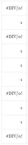
Now the formula =LOOKUP(2,1/(NOT(ISBLANK(A1:A10))), A1:A10) will be translated to =LOOKUP(2,{‘#DIV/0!’, 1, ‘#DIV/0!’, 1 , 1, 1, ‘#DIV/0!’, 1, 1, ‘#DIV/0!’}, A1:A10).
The excel lookup function will look for the first parameter value 2 in the second array list from the first array element to the last array element.
If it can not find the number value 2 until the last element in the second array list, it will return the last non-empty array element’s row number which is row 9.
Then the LOOKUP function will return the number 9th element ( A9 ) value ( Apple Watch ) in the third parameter ( A1:A10 ).
Besides the above formula, you can also use the formula =LOOKUP(0.1,0/(NOT(ISBLANK(A1:A10))), A1:A10) to get the last non-empty element, the principle is the same as the first formula.
If you want to get the last non-empty cell’s row number in this example.
You can use the formula =LOOKUP(2,1/(A1:A10<>””),ROW(A1:A10)) to implement it.
You can read the article Excel Table LOOKUP Function Examples to learn how to use the excel LOOKUP function.