How To Create A Drop Down List From Excel Table Column

In the previous article, I told you how to add a drop-down list in an Excel cell. In this article, I will tell you how to create a drop-down list from an Excel table column.

1. How To Create A Drop-Down List From Excel Table Column.

1.1 Create The Source Data Table Column.

1. Below is the example cell data column.
   
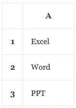
2. Select the cell range A1:A3, then click the Home tab —> Format as Table drop-down arrow in the Styles group, and select a table style to convert the column data to a table as below.
   
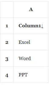
3. Select the above table, and click the Table Design tab ( this tab only appears when you select a table ), then get the table name from the Table Name text box in the Properties group.

1.2 Create A Drop-Down List From The Source Excel Table Column.

1. Select cell C1, and click the Data tab —> Data Validation↓ —> Data Validation menu item to open the Data Validation dialog.
2. Click the Settings tab, and select the item List from the Allow drop-down list.
3. Input the formula =INDIRECT(“Table-name[Column1]”) in the Source input text box.
4. Click the OK button to save the dialog settings.
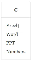
5. Now when you select cell C1, you can see a down arrow (↓) beside the cell.
6. When you click the down arrow, it will list all the cell data in Column1 of the source table.
7. You can right-click a cell in the source table, then click the menu item Insert —> Insert Rows Above to add a cell in the table column, and then input the cell data ( Numbers ) in it.
8. Now when you click the down arrow (↓) of the drop-down list in cell C1, you can find the newly added table column cell data in the list.
   

References

1. How To Add Drop Down List In Excel Cell.
2. How To Use Excel Indirect Function Examples.