How To Create, Remove Excel PivotTable Examples

In this article, I will tell you what is excel pivot table and how to create, and remove excel PivotTable with examples.

1. What is an Excel PivotTable?

1. An Excel PivotTable is a powerful feature that allows you to summarize and analyze large amounts of data in a spreadsheet.
2. It enables you to quickly create a summary report by grouping data into categories and displaying the results as a table.
3. PivotTables allow you to filter, sort, and manipulate data in a variety of ways, making it easy to identify trends, patterns, and outliers.
4. It is a useful tool for data analysis and reporting in Excel.

2. How To Create An Excel PivotTable Example.

1. Here is an example of how to create an Excel PivotTable.
2. We have a large dataset with sales information for a company as below.
3. This is a simple dataset that includes sales information for two product categories (Widgets and Gadgets) in two regions (East and West).
   
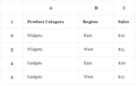
4. We want to analyze the sales by product category and region.
5. Here’s how we can create a PivotTable to do that.
6. Select the entire dataset, including headers.
7. Go to the “Insert” tab in the Excel ribbon and click on “PivotTable” in the Tables group.
8. It will pop up the PivotTable from table or range dialog window.
9. The cell range that you selected is inputted in the Table/Range text box.
10. And it checks the New Worksheet radio button by default.
11. If you check the Existing worksheet radio button, you should specify the existing worksheet name and the starting cell address such as ‘Sheet5’!$A$1.
12. Make sure the starting cell address does not overwrite the existing PivotTable in the existing worksheet.
13. Click the OK button, then it will create a new worksheet and display the PivotTable Fields pane on the excel right side.
14. In the PivotTable Fields pane, drag the “Product Category” field to the “Rows” area and the “Region” field to the “Columns” area.
15. Drag the “Sales” field to the “Values” area.
16. Excel will automatically create a table that shows the total sales for each product category and region.
17. You can further customize the table by adding filters, sorting, and formatting.
18. Here’s what the resulting PivotTable might look like.
    
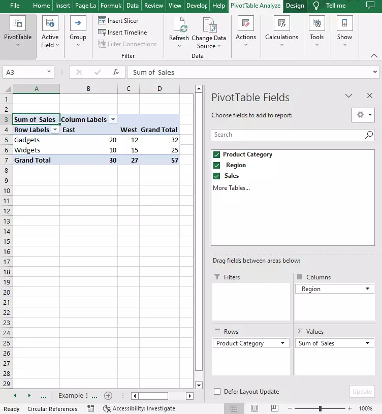
19. This PivotTable shows the total sales for each product category in each region, as well as the total sales for all regions.
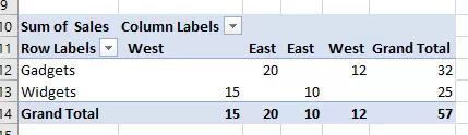
20. But you should note if the Region value contains hidden characters such as white space at the beginning or end, it will treat the value as a different region value.
21. For example, if one region value is “East “, and another region value is ” West “, the PivotTable will treat the region value as 2 new regions.
22. And you will get the PivotTable that is not correct like below.
    

3. How To Remove an Excel PivotTable?

1. To remove an Excel PivotTable, follow these steps.
2. Click anywhere inside the PivotTable to select it.
3. Click the “PivotTable Analyze” tab in the Excel ribbon.
4. Click on “Select” in the “Actions” group and choose “Entire PivotTable” to select the entire PivotTable.
5. Click the PivotTable Analyze tab —> Clear —> Clear All in the Actions group to remove the PivotTable.
6. Note that clearing a PivotTable will remove all the fields, formatting, and calculations associated with it.
7. There is also a quick and easy way to remove all the PivotTables in an excel worksheet, that is delete the newly created worksheet by right-clicking the worksheet name and then clicking the Delete menu in the popup menu list.