When I use wildcards in the excel VLOOKUP function to find a wanted cell value, I meet a strange issue. I found the wildcards are not working as I expected. This article will tell you how to fix the VLOOKUP wildcard not working issue.
1. VLOOKUP Wildcards Not Working Example 1.
1.1 Example Description.
- Below are the example data cells.
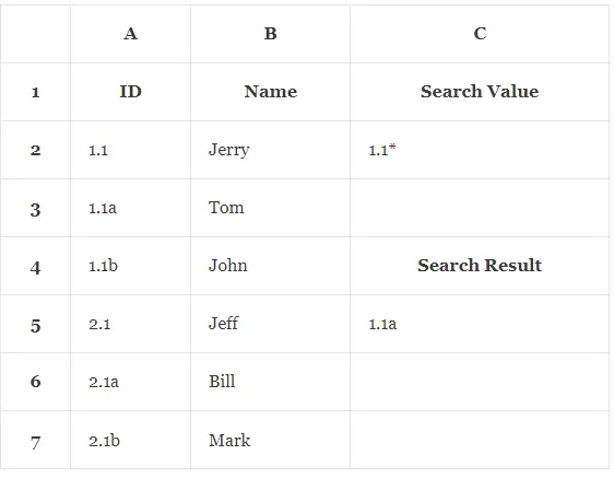
- There are 3 columns in the above data cells, column A is the ID list, column B is the Name list, and column C contains the Search Value and Search Result cell.
- The ID list contains values 1.1, 1.1a, 1.1b, 2.1, 2.1a, and 2.1b.
- The cell below the Search Result cell ( cell C5 ) contains the formula =VLOOKUP(C2, A2:B7,1, FALSE).
- When you input the search value 1.1* in cell C2, the formula in C5 will show the text 1.1a (cell A3‘s value).
- But this is not what I want, I want to show the text 1.1 (cell A2‘s value) in cell C5 because the wildcard * means zero or multiple characters.
1.2 How To Fix This Issue?
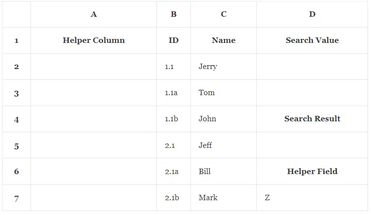
- Add the text Helper Field in cell C6, and input the character Z in cell C7, we will use this character as the helper character.
- Click to select column A and right-click the mouse pointer, then click the Insert menu item in the popup menu list to insert a new column.
- Now the other columns will move to the next column on the right side automatically.
- Add the text Helper Column in cell A1.
- Input the formula =CONCAT(B2,$D$7) in cell A2 and press the enter key, then it will show text 1.1Z in cell A2.
- The excel CONCAT function will add the inputted cell list values to a new value.
- Click to select cell A2, then click the small square on the bottom right corner of cell A2 and drag the mouse pointer to cell A7.
- Then it will autofill the formula to the cell range A2:A7, you can get the below table.
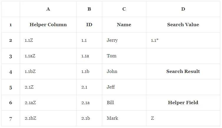
- Input the query string 1.1* in cell D2.
- Input the formula =VLOOKUP(D2, A2:B7,2, FALSE) in cell D5 and press the enter key, then it will show the value 1.1 which we wanted in cell D5.