When you draw a line graph in excel, you can choose to draw a line graph or a line graph with markers for each data point. In this article, I will tell you how to show or hide the lines between markers or markers only in excel line graph.
1. How To Show Hide Lines Or Markers In Excel Line Graph.
- Below is an excel combo chart, it contains one column chart and one line marker chart.
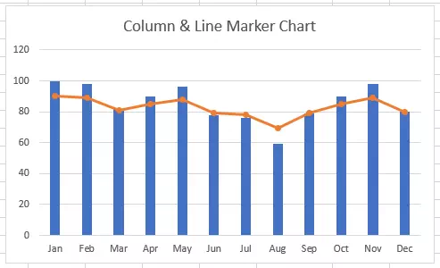
- This post will use the above combo chart as an example.
1.1 How To Show Or Hide Lines Or Markers In Line Marker Graph.
- The above line marker chart show it’s markers by default.
- If you want to hide the marker, you can double click the line marker graph to open the Format Data Series panel on excel right side.
- Click the Fill & Line icon ( a paint bucket ) in the Series Options section.
- There are 2 items under it, Line and Marker.
- When you click the Line item, there are 4 radio buttons, they are No line, Solid line, Gradient line, and Automatic.
- Select the No line radio button, then it will hide the lines between markers in the line marker graph and display the markers only.
- If you select other radio buttons, it will show the lines between the markers in the line marker graph accordingly.
- When you click the Marker item, it will display the marker related properties under it.
- Expand the Marker Options, it will display 3 radio buttons, they are Automatic, None, and Build-in.
- Select the None radio button will hide the markers in the line marker graph.
- Select the other radio buttons will show the markers in the line marker graph.