How To Sort Rows By Multiple Columns In Excel And Vice Versa

In this article, I will tell you how to sort excel table rows by one column or multiple columns value in descending or ascending order. You can also use this method to sort excel table columns by one row or multiple rows value.

1. How To Sort Excel Table Rows By Multiple Columns Value Steps.

1. Here are the steps to sort an Excel table rows by one column value.
2.  Select the entire table by clicking on the box to the left of the column headers and above the row numbers. Alternatively, you can press “Ctrl+A” on your keyboard to select the entire table.
3. Click on the “Data” tab in the Excel ribbon.
4. In the “Sort & Filter” group, click on the “Sort Smallest to Largest (A -> Z)” or “Sort Largest to Smallest (Z -> A)” button, depending on how you want to sort the table.
5. Then it will popup the Sort dialog window.
   
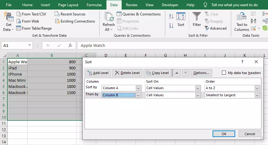
6. By default, it will sort the rows by columns, you can select the sorted column in the Sort by drop-down list.
7. If you want to add a second level sort column after the first column, you can click the Add Level button to add a new sort condition.
8. One line of the Sort by condition contains the Column name, Sort On, and Order.
9. The Sort On drop-down list contains 4 values which are Cell Values, Cell Color, Font Color, and Conditional Formatting Icon.
10. The Order drop-down list contains 3 values which are A to Z, Z to A, Smallest to Largest, Largest to Smallest, and Custom List….
11. If you select the order item Custom List…, it will popup the Custom Lists dialog window, you can specify your custom list in the dialog window.
12. Now you can click the OK button to implement the sort operation.
13. Then you will find the excel dataset will be sorted by the selected multiple columns values and orders.

2. How To Sort Excel Table Columns By Multiple Rows Value Steps.

1. If you want to sort the excel table column by multiple rows value, you can click the Options… button on the top right corner of the above Sort dialog window.
2. Then it will popup the Sort Options dialog window.
3. Check the radio button Sort left to right and click the OK button.
4. Then the Sort by drop-down list items in the Sort dialog will be changed to the table’s rows name such as Row 1, Row 2, ….
5. If you select the radio button Sort top to bottom in the Sort Options dialog window.
6. It will sort the table data by columns value, then the Sort by drop-down list items in the Sort dialog will be changed to the table’s column’s name such as Column A, Column B, ….

3. How To Open The Sort Dialog Window In Another Way.

1. Select one column or row in excel table.
2. Click on the “Data” tab in the Excel ribbon.
3. In the “Sort & Filter” group, click on the “Sort Smallest to Largest” or “Sort Largest to Smallest” button, depending on how you want to sort the table.
4. In the “Sort Warning” dialog box, select “Expand the selection” and click the “Sort…” button.
5. Then it will open the Sort dialog window.