The excel HLOOKUP function is similar to the VLOOKUP function. It can look up a value in the first row of an excel cell range horizontally. When it finds the matched cell then it will return the cell value in the row specified by the row index number of the cell range. The returned cell is in the same column as the matched cell in the cell range’s first row.
1. Excel HLOOKUP Function Introduction.
- Below is the excel HLOOKUP function’s syntax. It is similar to the VLOOKUP function, the only difference is the lookup direction is horizontal.
=HLOOKUP(lookup_value, table_array, row_index, [range_lookup])
- lookup_value: the value that you want to look up in the first row of the specified cell range.
- table_array: the look-up cell range. The HLOOKUP function will search the value in the first row of the table_array.
- row_index: the result row index number in the table_array. When the HLOOKUP function finds the lookup_value in the first row of the table_array, then it will return the cell in the row specified by the row_index number.
- range_lookup: the boolean value, TRUE means approximate match, FALSE means exact match. It is the same as the VLOOKUP function, you can refer to the article Excel Vlookup Approximate Match And Exact Match Example.
- When you implement the exact match ( pass FALSE to the range_lookup parameter ), you can use the wildcards to implement a fuzzy match. Please read the article How To Use Vlookup Wildcard To Implement Partial Match In Excel, How To Fix Vlookup Wildcard Not Working Issue.
2. Excel HLOOKUP Function Example Data Cells.
- Below is the example data cell table.
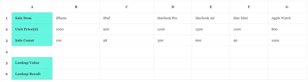
- Row A1:G1 is the Sale Item row, row A2:G2 is the Unit Price($) row, and row A3:G3 is the Sale Count row.
- You can first create a vertical cell table and then transpose it to the horizontal cell table like the above. You can read the article How To Transpose Rows And Columns In Excel Table to learn more.
- In this example, you can input the look-up value in cell B5.
- And then input the formula in cell B6.
3. Excel HLOOKUP Formula Example.
- Input the formula =HLOOKUP(B5, A1:G3, 3,FALSE) in cell B6. Below is the formula argument explanation.
- B5: The cell contains the look-up value.
- A1:G3: The cell range that contains the look-up value row and the result row.
- 3: When it finds a matched cell in the first row ( A1:G1 ), then it will return the cell ( in the same column as the matched cell ) in the third ( specified by the number 3 ) row ( A3:G3 ).
- FALSE: Means exact match.
4. How To Implement Exact Lookup Using HLOOKUP Function.
- Now input the lookup value Apple Watch in cell B5, then it will show the value 1000 in cell B6. The number 1000 ( in cell G3 ) is the Apple Watch‘s sale count.
- Input the look-up value iP* in cell B5, then it will show the number 100 in cell B6. The number 100 ( in cell A3 ) is the iPhone‘s sale count.
- Input the look-up value iPa? in cell B5, then it will show the number 98 in cell B6. The number 98 ( in cell B3 ) is the iPad‘s sale count.
5. How To Implement Approximate Lookup Using HLOOKUP Function.
- When you change the formula to =HLOOKUP(B5, A1:G3, 3, TRUE) in cell B6, it will implement an approximate lookup ( the fourth parameter is TRUE ).
- But you should sort the cells in the first row A1:G1 in ascending order before you can implement the approximate lookup ( please refer to the article Excel Sort Rows By Column Value Example ).
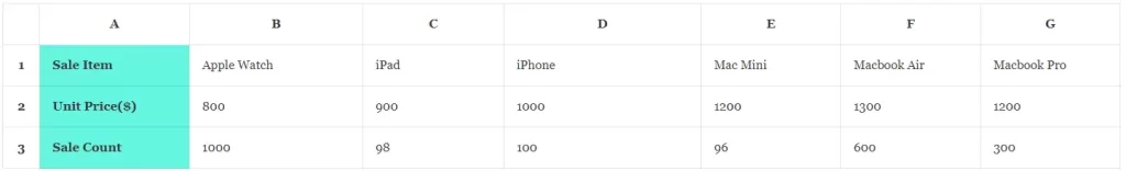
- Now input the text Mac Mkx in cell B5, it will show the number 96 in cell B6.
- This is because the function can not find the exact text Mac Mkx in row A1:G1, but it will implement an approximate match (because the fourth argument is TRUE ), so it will not return the error text #N/A.
- It finds the text Mac Mini is the closest text which is smaller than the lookup text Mac Mkx, so cell E1 contains the approximate text to the lookup value Mac Mkx.
- So it will return the cell E3‘s value ( 96 ) because the third argument is 3 which points out to return the third row in the cell range.