How To Use Excel Index Function With Examples

The Excel INDEX function is used to find a value in a specified array or one/multiple cell ranges. This article will tell you how to use the Excel index function to find data with some examples.

1. Excel INDEX Function Syntax.

1. The Excel INDEX function has the below function syntax.

   INDEX(array, row_num, [column_num])
   
   or
   
   INDEX(reference, row_num, [column_num], [area_num])
   

2. The INDEX function has 3 or 4 arguments, the first argument is an array or cell ranges reference.
3. The cell ranges reference can contain one or multiple cell ranges such as (A1:B6, E1:F6, I1:J6).
4. The second argument row_num specifies the row number of the returned element located in the array or cell range.
5. The third argument column_num specifies the column number of the returned element located in the array or cell range.
6. If the first argument is a multiple cell ranges reference, then the fourth argument area_num points out which cell range in the multiple cell ranges is used to locate and return the value.
7. If you pass 0 to the row_num argument, then it will return the entire column data specified by the column_num argument.
8. If you pass 0 to the column_num argument, then it will return the entire row data specified by the row_num argument.

2. Excel Index Function Examples.

2.1 Using Excel Index Function To Get Data From Array Example.

1. Input the formula =INDEX({1,2,3;4,5,6;7,8,9},0,3) in cell A1 and press enter key, then it will display the data 3,6,9 in column cell range A1:A3.
2. Input the formula =INDEX({1,2,3;4,5,6;7,8,9},3,3) in cell A1 and press enter key, then it will display the data 9 in cell A1.
3. Input the formula =INDEX({1,2,3;4,5,6;7,8,9},3,0) in cell A1 and press enter key, then it will display the data 7,8,9 in row cell range A1:C1.
4. Input the formula =INDEX({1,2,3;4,5,6;7,8,9},3) in cell A1 and press enter key, then it will display the data 7,8,9 in cell range A1:C1.
5. Input the formula =INDEX({1,2,3,4,5,6,7,8,9},6) in cell A1 and press enter key, then it will display number 6 in cell A1.

2.2 Using Excel Index Function To Get Data From Cell Ranges Example.

1. Below are the example data cells.
   
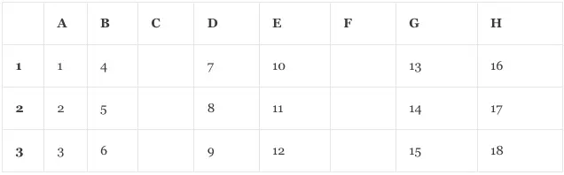
2. There are 3 rows and 8 columns in the above data cells.
3. Columns C and F are 2 empty columns. Now we will use the Excel INDEX function to get the element in the above data cells.
4. The formula =INDEX(A1:B3,1,0) will return the first row in cell range A1:B3, it will return the cell range A1:B1 which contains the number 1,4.
5. The formula =INDEX(A1:B3,1,1) will return the first cell A1 which contains the number 1.
6. The formula =INDEX(A1:B3,0,1) will return the first column in cell range A1:B3, it will return the cell range A1:A3 which contains the number 1,2,3.
7. The first argument of the INDEX function can be multiple cell ranges such as (A1:B3, D1:E3, G1:H3).
8. And in this case, you should pass the fourth argument area_num to point out which cell range is used to find the cell value by the row_num and column_num address.
9. For example, the formula =INDEX((A1:B3, D1:E3, G1:H3), 0,1,2) will return the first column in the cell range D1:E3.
10. This is because the last argument ( area_num ) is 2 in the above formula, then it will use the second cell range in the first argument (A1:B3, D1:E3, G1:H3).
11. In this example, the above formula will return the column cell range D1:D3 which contains the number 7,8,9.
12. Please note, if you use the formula =INDEX((A1:B3, D1:E3, G1:H3), 0,3,2), then it will throws the #REF! error, this is because the cell range D1:E3 only contains 2 columns but the above formula requires the third column in cell range D1:E3.