In the previous article, I told you how to use the excel advanced filter and the remove duplicate menu to remove duplicate rows in excel. In this article, I will tell you how to use a formula to filter out duplicate rows in excel and remove them.
1. How To Use Formula To Remove Duplicate Rows In Excel.
- We use the below data example, there are duplicate rows in it.
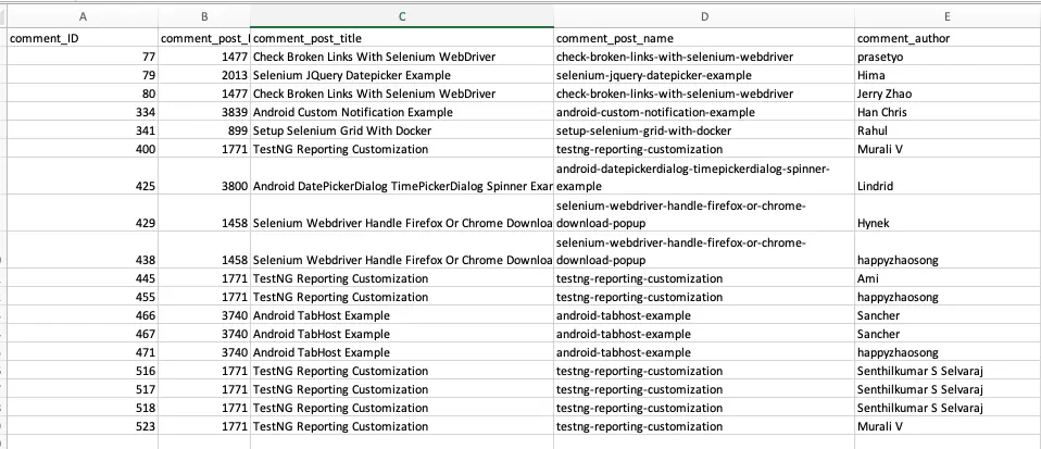
- Now we will filter out the rows in which columns C, D, and E contain duplicate data, which means when 2 rows contain the same data in columns C, D, and E, the 2 rows are treated as duplicates.
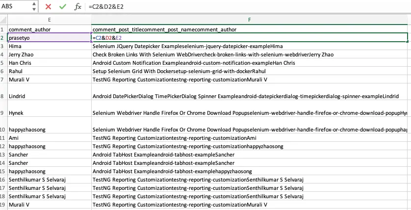
- Input the formula = C2&D2&E2 in cell F2, then autofill the formula in column F until the last row.
- Then it will combine the data in columns C, D, and E and put the result in column F.
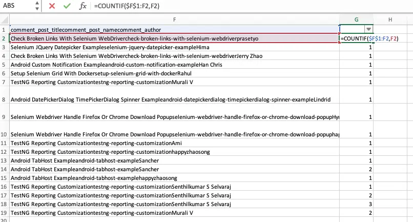
- Now, input the formula =COUNTIF($F$1:F2, F2) in cell G2, and auto-fill the formula in column G until the last row.
- Then it will count and display the number of times the cell data appears in column F, you can see some data appears more than one time.
- Select column G and click the excel Data —> Filter menu item to open the Filter dialog window.
- Check the checkbox before the number 1 in the column data list of the Filter area.
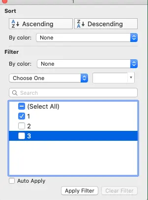
- When you click the Apply Filter button, it will display the rows that column G contains the number 1 only.
- In such a way, it filters out and removes the duplicated rows in the example dataset, you can copy the unique rows and paste them into another excel worksheet.