Excel Table Lookup Function Examples

This article will tell you how to use the excel LOOKUP function to look up the provided value in a table column and return the first matched cell data in the same or another column. It will provide several examples to show the use cases. The LOOKUP function is supported in all excel versions.

1. Excel LOOKUP Function Introduction.

1. Below is the excel LOOKUP function syntax.

   =LOOKUP(lookup_value, lookup_vector, [result_vector])
   

2. The excel LOOKUP function will search the lookup_value ( the first parameter ) in the lookup_vector ( the second parameter ).
3. If found then return the related cell value from the result_vector or the lookup_vector ( if do not provide the result_vector ).
4. lookup_value: the search value in the lookup_vector.
5. lookup_vector: can be one row or one column cell range in where to search the lookup_value.
6. Before you call the excel LOOKUP function, you must sort the lookup_vector element in ascending order.
7. result_vector: the one-row or one-column cell range that contains the result cell. This parameter is optional, if you do not provide this parameter, it will return the matched cell in the lookup_vector.
8. The lookup_vector and the result_vector must have the same size.
9. The LOOKUP function is case-insensitive, which means that searching the lookup value apple or APPLe will return the same result.
10. If the LOOKUP function finds that the lookup_value is greater than any value in the lookup_vector, then it will match the lookup_vector‘s last value.
11. If the LOOKUP function finds that the lookup_value is smaller than any value in the lookup_vector, then it will return the error #N/A.
12. If the function can not find the lookup_value in the lookup_vector, it will match the value that is smaller than the lookup_value in the lookup_vector. And then return the mapped cell value in the result_vector.

2. Excel LOOKUP Function Examples.

2.1 Example Data Table.

1. Below is the article’s example data table.
   
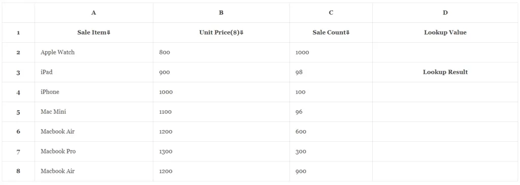
2. First, you should make sure that you have converted the above data cells to an excel table so that you can sort the lookup_vector column or row in ascending order. Please refer to the article Excel Convert Table To Range Example And Vice Versa.

2.2 Sort The lookup vector Column In Ascending Order.

1. We will use column A as the lookup_vector, so click the down arrow after the title Sale Item and click the Sort A to Z item in the popup menu list to sort column A in ascending order.

2.3 Input The Formula Using The Excel LOOKUP Function.

1. Input the formula =LOOKUP(D2, A2:A8, A2:A8) in cell D4, then it will lookup the cell D4‘s value in cell range A2:A8, and then return the related cell value in cell range A2:A8 in the founded row.
2. In the above formula, we use the cell range A2:A8 as the lookup_vector and result_vector, you can use a different cell range.

2.4 The LOOKUP Function Is Case Insensitive.

1. Now input the lookup value aPPLE watCH in cell D2, then you can find it will show the text Apple Watch in cell D4.
2. This confirms the LOOKUP function is case insensitive.

2.5 Return Error Text When The Lookup Value Is Smaller Than Any Cell Value.

1. Input the lookup value alphabet in cell D2, it will show the error text #N/A in cell D4.
2. This is because it can not find the lookup_value alphabet in column A and the lookup_value alphabet is smaller than the first cell’s value Apple Watch in alphabetic order.

2.6 Return The Nearest Smaller Cell Value When Can Not Found The Lookup Value.

1. Input the lookup value Lenovo in cell D2, it will show the text iPhone in cell D4.
2. This confirms when it can not find the exactly matched cell value ( Lenovo ), it will return the nearest smallest cell value. And the value iPhone is just the nearest smallest value in column A.

2.7 Return The Last Cell Value When The Lookup Value Is Greater Than All the Cell Values In The Lookup Vector.

1. Input the lookup value Nokia in cell D2, it will show the text Macbook Air in cell D4.
2. This is because no cell in column A contains the value Nokia, and the lookup_value Nokia is greater than all the cell values in column A, so it returns the last cell value.

2.8 Implement Right To Left Lookup.

1. The formula =LOOKUP(D2, A2:A8, C2:C8) will look up the cell D2‘s value in cell range A2:A8 and return the related cell value in cell range C2:C8. This is the so-called Left-to-Right lookup.
2. And the LOOKUP function can also implement Right-to-Left lookup, the formula =LOOKUP(98, C2:C8, A2:A8) will lookup the number 98 in cell range C2:C8 and return the related cell in cell range A2:A8. In this example, it will return the text iPad. But first, you should sort column C in ascending order.