How to Create a Scrolling Chart in Excel: A Step-by-Step Guide with Examples

In today’s data-driven world, visualizing information is key to understanding trends and making informed decisions. Excel, with its powerful charting capabilities, allows users to create dynamic and interactive charts that can effectively communicate insights. One such chart type is the scrolling chart, which enables users to display a large dataset within a limited space while maintaining clarity and readability. In this article, we’ll walk through the process of creating a scrolling chart in Excel, supplemented with examples and a sample dataset.

1. Sample Dataset.

1. To illustrate the creation of a scrolling chart, let’s consider a hypothetical dataset representing monthly sales figures for a fictional company.
2. The dataset consists of two columns: “Month” and “Sales Amount“.
3. Here’s a sample dataset that you can copy into separate columns in Excel:

   Month     Sales Amount
   Jan       10000
   Feb       12000
   Mar       15000
   Apr       11000
   May       13000
   Jun       14000
   Jul       16000
   Aug       17000
   Sep       18000
   Oct       20000
   Nov       19000
   Dec       22000
   

1. Prepare Your Data.

1. Before creating the scrolling chart, ensure that your data is organized properly in Excel.
2. In our example, the “Month” column serves as the x-axis labels, while the “Sales Amount” column represents the y-axis values.

2. Insert a Scroll Bar Control.

1. To create the scrolling functionality, we’ll use Excel’s Form Control called the Scroll Bar.
2. To insert a Scroll Bar, follow the below steps.
3. Go to the “Developer” tab (if not visible, enable it in Excel options).
4. In the “Form Controls” section, select “Scroll Bar“.
5. Click and drag to draw the scroll bar on your worksheet.

3. Set Properties of the Scroll Bar.

1. After inserting the scroll bar, you need to set its properties to control its behavior.
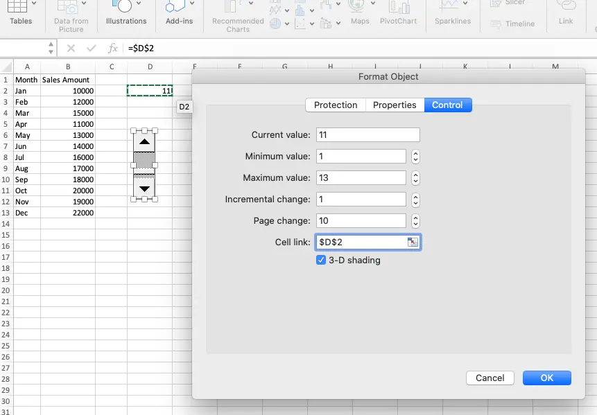
2. Right-click on the scroll bar and select “Format Control“.
3. You can do the following in the Format Control dialog box:
4. Set the “Minimum Value” to 1 (the first row of data).
5. Set the “Maximum Value” to the number of rows in your dataset.
6. Set the “Incremental Change” to 1 (scrolls one row at a time).
7. Optionally, adjust other properties such as cell link and orientation.

4. Change the Scroll Bar Orientation.

1. If you want to change the scroll bar orientation, just resize it.
2. If you make the scroll bar height bigger than it’s width, then the scroll bar is a vertical scroll bar.
3. If you make the scroll bar width bigger than it’s height, then the scroll bar is horizontal.

5. Link the Scroll Bar to a Cell.

1. To make the scroll bar interact with your data, you need to link it to a cell. This cell will contain the value corresponding to the current position of the scroll bar.
2. Right-click on the scroll bar, select “Format Control” and specify the cell reference under “Cell link“.
3. In this example, we select cell $D$2 as the cell link value, so the scroll bar current value will be reflected on cell D2.
   

6. Create a Dynamic Range for Chart Data.

1. To ensure that the chart displays only the visible portion of the dataset based on the scroll bar’s position, you need to create a dynamic range using Excel’s OFFSET or INDEX functions.
2. For our example, let’s use the OFFSET function:

   `=OFFSET($B$2,$D$2-1,0,10,1)`

3. Here, `$B$2` is the starting cell of the “Sales Amount” column, `$D$2` is the cell linked to the scroll bar, `10` is the number of rows to display, and `1` is the number of columns.
4. Understand the OFFSET Function Parameters.

   - `reference`: The starting point or reference cell.
      - `rows`: The number of rows to offset from the reference cell. In our case, we're subtracting 1 from the scroll bar value to align with Excel's indexing (rows start from 1).
      - `cols`: The number of columns to offset from the reference cell (0 in this case).
      - `height`: The height, in number of rows, that you want the range to be.
      - `width`: The width, in number of columns, that you want the range to be (1 in this case since we're selecting a single column).

5. Begin by selecting the range of data you want to make dynamic. In our example, select the range of sales data including headers (“Month” and “Sales Amount“).
6. Click on the cell where you want to display the dynamic range. For example, if you want the dynamic range to start from cell E2, click on cell E2.
7. After entering the formula, press Enter. You’ll see the dynamic range now displays the portion of data corresponding to the current position of the scroll bar.
8. When you click the arrow on the scroll bar, the range value will also change accordingly.

7. Create a Chart.

1. With the dynamic range set up, you can now create your chart.
2. Select the dynamic range of data (including the x-axis labels), go to the “Insert” tab, and choose your desired chart type (e.g., line chart, column chart).
   

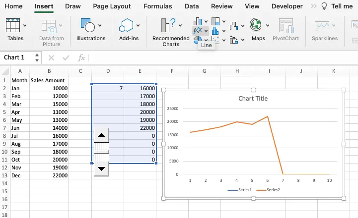
8. Test the Scrolling Functionality.

1. Once the chart is created, test the scrolling functionality by interacting with the scroll bar.
2. As you move the scroll bar, the chart should update to display the corresponding portion of the dataset.

9. Conclusion.

1. In this tutorial, we’ve explored how to create a scrolling chart in Excel to visualize large datasets effectively.
2. By following the step-by-step guide and using the provided examples, you can harness Excel’s features to present your data dynamically and enhance decision-making processes.
3. With the ability to scroll through extensive datasets while maintaining clarity and readability, scrolling charts offer a versatile solution for data visualization in Excel.
4. Experiment with different chart types, formatting options, and dataset sizes to create compelling visualizations tailored to your specific needs.