How To Use Excel Autosum Example

In the previous article, I told you how to use the Excel SUM function to add multiple cell number values in the formula. In this article, I will tell you how to use a shortcut button ( ∑ AutoSum button ) to summarize a column or a row of cell number values quickly, easily, and automatically.

1. How To Autosum A Column In Excel.

1. Below are the example data cells.
   
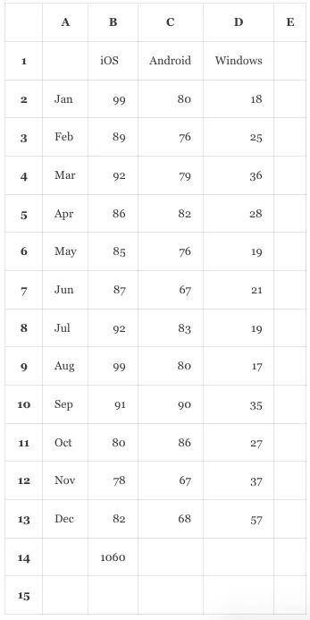
2. If you want to summarize column B‘s number, you can select cell range B2:B13 and then click the Formulas tab on the Excel top menu bar.
3. Then click the AutoSum item ( ∑ item ) in the Function Library group.
4. Then you will find it adds all the number values in the cell range B2:B13 and puts the number in cell B14 automatically.
5. If you select cell B14, you can find it adds the formula =SUM(B2:B13) in the cell automatically.
6. You can use the Excel Autosum function in another way.
7. Click the cell C15, then click the Formulas tab —> ∑AutoSum item in the Function Library group.
8. Then it will show a dotted box around the cells above cell C15.
   
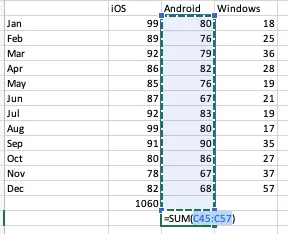
9. If you confirm the cell range in the dotted box is correct, you can press the enter key to enter the formula in cell C15.
10. Then you can see the column number summary in cell C15 also.
11. The Excel Autosum function will select and summarize the cells above ( not below ) the selected cell, and it will stop at the cell that contains a non-numeric value ( text, date, blank).
12. But you can adjust the selected cell range by dragging the dotted box corner square to include the non-numeric cells.
13. When you drag the dotted box border to change the cell range, you can find the formula contained in cell C15 is changed accordingly.
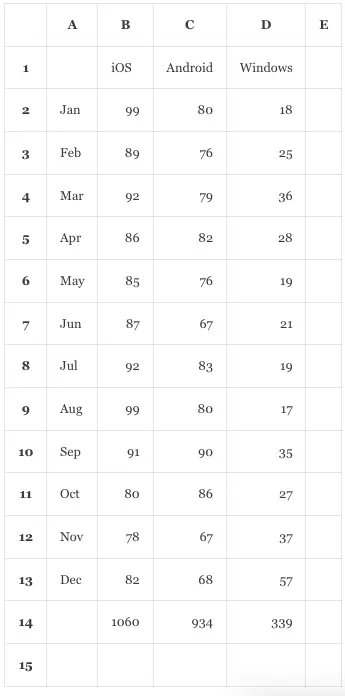
14. If you want to summarize the 3 columns (columns B, C, D ) at the same time, you can select cell range B2:D13 to select all the 3 columns at the same time.
15. Then click the Formulas tab —> ∑ AutoSum item to summarize all the 3 columns’ numbers and display the result in the last empty row.
    
16. There is another method to auto-summarize the 3 column’s numbers at a time.
17. Select the empty cell range B15:D15, there are 3 cells in the range B15, C15, and D15.
18. Then click the Formulas tab —> ∑ AutoSum item, then it will summarize the 3 column numbers and put the result in cell range B15:D15.

2. How To Autosum A Row In Excel.

1. Select the cell range B2:D2 in the above example row 2.
2. Then click the Formulas tab —> ∑ AutoSum item will summarize the above row numbers and put the result in cell E2.
3. You can use the above method to process each row of data one by one, but it is not efficient.
4. There is another method to auto-summarize multiple rows of numbers easily.
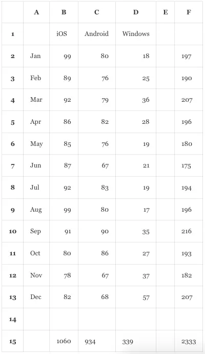
5. In this example, select the cell range B2:F15 and click the Formulas tab —> ∑ AutoSum item.
6. Then it will summarize each row and column’s numbers automatically and put the result at the end of each row and column.
7. It will also auto-summarize all the cell numbers in the cell range and put the result in cell F15 at the bottom right corner of the cell range.