How To Use Excel SUMPRODUCT Formula Example

The Excel function SUMPRODUCT is very useful when you want to use a formula to calculate the summary of multiple number arrays. This article will tell you how to use the Excel SUMPRODUCT formula with examples.

1. The Excel SUMPRODUCT Function Syntax.

1. Below is the syntax of the Excel function SUMPRODUCT.

   SUMPRODUCT(Array1, [Array2], [Array3],…)

2. The first array of the SUMPRODUCT function can not be omitted. All the arrays should have the same size.
3. The function will multiply all the elements in the multiple array accordingly and then summarize each result and return the number.
4. For example, input the formula =SUMPRODUCT({1,2,3},{4,5,6}) in any Excel worksheet cell and press enter key, then it will display the number 32 in the cell.
5. The above formula will calculate the 2 arrays as 1*4+2*5+3*6 = 4+10+18=32.
6. If you just pass one array to the Excel function SUMPRODUCT in a formula such as =SUMPRODUCT({1,2,3}), then it will add all the numbers in the array and return the result number 6 ( 1 +2 +3 ).

2. How To Use Excel SUMPRODUCT Formula To Calculate Total Sales Revenue.

1. Below are the example data cells.
   
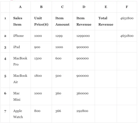
2. Column A contains the item name, column B contains the item unit price, and column C contains the item amount.
3. If we want to calculate the total revenue of all the sales items, we need to calculate each item’s revenue by Unit Price * Item  Amount, then add up all the item’s sales revenue together.
4. We can input the formula =B2*C2 in cell D2 and press the enter key, then it will display the result number in cell D2.
5. Select cell D2, and drag the small square on the bottom right corner of the cell to cell D7.
6. Then it will auto-fill the same formula to each of the cells in cell range D3:D7, but the formula will change the cell number in the formula to the current row number.
7. For example, the formula will be changed to =B3*C3 in cell D3, and be changed to =B6*C6 in cell D6 .etc.
8. Input the formula =D2+D3+D4+D5+D6+D7 in cell F2 and press enter, it will display the number 4651800 in this cell.
9. If we use the Excel SUMPRODUCT function to implement this, we can input the formula =SUMPRODUCT(B2:B7, C2:C7) in cell F1.
10. When we press the enter key, it will show the same number as in cell F2, so this can confirm the calculated result number is the same and correct.

3. How To Use Excel SUMPRODUCT Formula To Calculate For Sales Item Revenue.

1. Now we add a column For Sale in the above sales table like below.
   
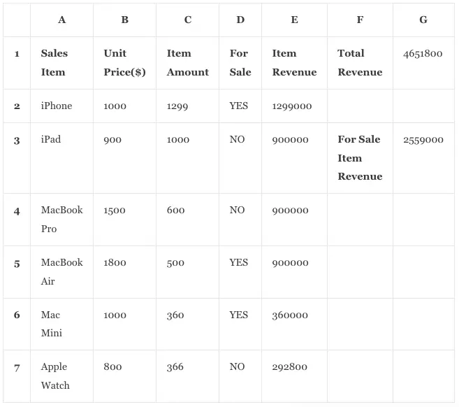
2. If the for sale column’s cell value is YES then it means the item is ready for sale, if the value is NO then it means the item is not ready for sale.
3. We want to calculate the For Sale Item Revenue in cell G3, so we can input the formula =SUMPRODUCT(–(D2:D7=”YES”),B2:B7,C2:C7) in cell G3 and press the enter key, then it will summarize the item revenue which is ready for sale in cell G3, you can see the number 2559000 in cell G3.
4. We will explain the formula step by step. The expression (D2:D7=”YES”) will return an array of Boolean values, you can input the formula =D91:D96=”YES” in any cell to get the Boolean array {TRUE, FALSE, FALSE,TRUE, TRUE, FALSE}.
5. When you input the formula =-(D2:D7=”YES”) in any cell, it will convert the Boolean array to a number array {-1,0,0-1,-1,0}.
6. We need positive numbers in the array, so we add a minus character before the above expression, you can change the above formula to =–(D2:D7=”YES”), it will return a positive number array {1,0,0,1,1,0}.
7. Now the formula =SUMPRODUCT(–(D2:D7=”YES”),B2:B7,C2:C7) will be changed to=SUMPRODUCT({1,0,0,1,1,0},B2:B7,C2:C7), it will multiply the 3 arrays elements accordingly and return the summarized result number.