How to Dynamically Extract Data Using Nested INDEX MATCH Formulas

Extracting data dynamically from a dataset based on multiple criteria can be efficiently achieved in Excel using a combination of INDEX, and MATCH. This article will guide you through constructing a formula that dynamically extracts the correct values from a dataset, ensuring accuracy and scalability.

1. Understanding the Dataset Structure.

1. Let’s consider a dataset structured as follows:

   | Month  | PID | Metric | Value |
   |--------|-----|--------|-------|
   | Jan    | 101 | A      | 15    |
   | Jan    | 101 | B      | 20    |
   | Jan    | 102 | A      | 25    |
   | Jan    | 102 | B      | 30    |
   | Feb    | 101 | A      | 18    |
   | Feb    | 101 | B      | 22    |
   | Feb    | 102 | A      | 28    |
   | Feb    | 102 | B      | 33    |
   

2. We aim to populate a “Result” column based on matching criteria in each row (Month, PID, and Metric), ensuring the formula adjusts dynamically as we fill it down.

2. Constructing the Formula.

1. To achieve this, we’ll use a combination of INDEX and MATCH functions, taking advantage of nested MATCH functions for multiple criteria matching.
2. Here’s the formula to be used in the “Result” column:
   

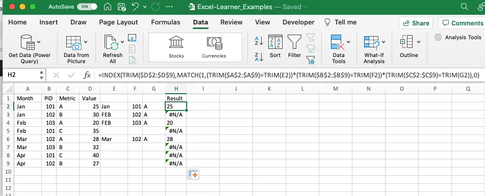
   =INDEX(TRIM($D$2:$D$9),MATCH(1,(TRIM($A$2:$A$9)=TRIM(E2))*(TRIM($B$2:$B$9)=TRIM(F2))*(TRIM($C$2:$C$9)=TRIM(G2)),0))

3. Let’s break down the formula step by step: This formula is designed to dynamically extract data from a table based on multiple criteria using the INDEX and MATCH functions. It also utilizes the TRIM function to remove any leading or trailing spaces that might cause discrepancies in comparisons.
4.  INDEX Function:– The `INDEX` function returns the value of a cell in a specific row and column of a range.
   – `INDEX(TRIM($D$2:$D$9), …)` specifies the range `$D$2:$D$9` containing the values to be retrieved. The `TRIM` function is used to remove any leading or trailing spaces from the values in this range.
5.  MATCH Function:– The `MATCH` function searches for a specified value in a range and returns the relative position of that value.
   – `MATCH(1, …, 0)` searches for the value `1` within the array generated by the logical conditions.
   – The logical conditions inside the `MATCH` function generate an array of TRUE/FALSE values based on whether the criteria match the values in the dataset.
6.  Logical Conditions:– `(TRIM($A$2:$A$9)=TRIM(E2))`: Compares each value in the range `$A$2:$A$9` (containing the “Month” column) with the value in cell `E2`. The `TRIM` function ensures that any leading or trailing spaces are removed before comparison.
   – `(TRIM($B$2:$B$9)=TRIM(F2))`: Compares each value in the range `$B$2:$B$9` (containing the “PID” column) with the value in cell `F2`.
   – `(TRIM($C$2:$C$9)=TRIM(G2))`: Compares each value in the range `$C$2:$C$9` (containing the “Metric” column) with the value in cell `G2`.
   – These comparisons generate arrays of TRUE/FALSE values, where TRUE indicates a match between the corresponding value in the dataset and the criteria specified in cells `E2`, `F2`, and `G2`.
7.  Multiplication of Logical Conditions:– The multiplication (`*`) of these logical conditions creates a combined array of TRUE/FALSE values.
   – This combined array ensures that only rows where all criteria match will have a TRUE value.
8.  MATCH Result:– The `MATCH` function returns the position of the first `1` (TRUE) found in the combined array.
   – This position corresponds to the row in the dataset where all criteria match.
9.  INDEX Result:– Finally, the `INDEX` function retrieves the value from the “Value” column (range `$D$2:$D$9`) corresponding to the row position determined by the `MATCH` function.
10. In summary, this formula dynamically extracts data based on multiple criteria while handling any leading or trailing spaces in the dataset and criteria values.
11. Below is the example in the Excel worksheet.
    

3. Conclusion.

1. With this formula, you can dynamically extract data based on nested criteria, ensuring accuracy and scalability as you fill it down.
2. Utilizing INDEX and MATCH functions in Excel provides a robust solution for handling complex lookup requirements efficiently.