How To Make A 3 Dimensional Chart In Excel With Examples

Excel is a powerful tool that can be used to create charts and graphs for data visualization. Among the various types of charts available in Excel, 3-dimensional (3D) charts are visually appealing and provide an engaging way to present data. In this article, we will explore how to make a 3D chart in Excel with examples.

Table of Contents

1. How To Make A 3 Dimensional Chart In Excel Steps.

Before we get started, it’s important to note that 3D charts have some limitations.
They can be difficult to read and interpret if there is too much data.
Additionally, they may not be compatible with all devices, such as small screens or projectors.
With those caveats in mind, let’s dive into creating 3D charts in Excel.

1.1 Step 1: Selecting the Data.

The first step is to select the data you want to use for your chart.
This can be done by highlighting the cells containing your data.
It’s also important to label your data with appropriate headers so that Excel can correctly identify what each column and row represents.

1.2 Step 2: Creating the Chart.

Once you’ve selected your data, click on the “Insert” tab in the top menu.
From there, select Recommended Charts button from the “Charts” group to open the Insert Chart dialog window.
Click the All Charts tab in the pop-up window.
You will see a variety of chart types, including 3D options on each chart type top area.
Choose the specific 3D chart type that best represents your data.

1.3 Step 3: Formatting the Chart.

After creating the chart, you can format it to better suit your needs.
This includes changing the chart title, axis labels, and adjusting the legend.
You can also change the colors and fonts used in the chart to match your existing branding or aesthetic.

1.4 Step 4: Adding Additional Data.

If you need to add additional data to your chart, you can do so by selecting the chart and clicking on the “Design” tab in the top menu.
From there, select “Select Data”.
This will allow you to add or remove data from your chart as needed.

2. How To Make A 3 Dimensional Chart In Excel Examples.

2.1 Example 1: 3D Column Chart.

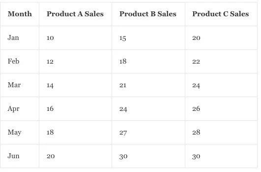
Let’s say you have data representing the sales of three different products over a period of six months.
You want to create a 3D column chart to represent this data visually.
First, select the data and click on the “Insert” tab.
From there, select “Column” under the “Charts” section.
Choose the 3D Clustered Column chart option.
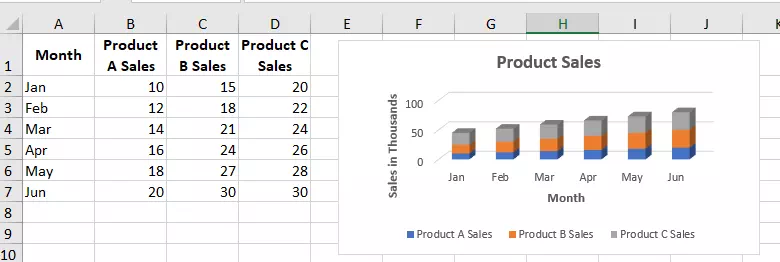
Next, format the chart by adding a title (“Product Sales”), labeling the X-axis (“Month”), and labeling the Y-axis (“Sales in Thousands”).
You can also adjust the legend and colors used in the chart to match your branding.
Finally, save and share the chart as needed.
Below is the example data.
Below is the 3D column chart created with the above example cell data.

2.2 Example 2: 3D Pie Chart.

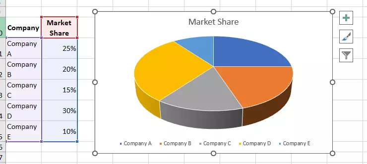
Let’s say you have data representing the market share of five different companies like below.
You want to create a 3D pie chart to represent this data visually.
First, select the data and click on the “Insert” tab.
From there, select “Pie” under the “Charts” section.
Choose the 3-D Pie chart option.
Next, format the chart by adding a title (“Market Share”), adjusting the legend position, and changing the colors used in the chart to match your branding.
Finally, save and share the chart as needed.

3. Conclusion.

Creating 3D charts in Excel is a powerful way to visualize data and make it more engaging for others to understand.
By following the steps outlined above, you can easily create your 3D charts and customize them to meet your specific needs.
Just remember to keep in mind the limitations of 3D charts and ensure they are appropriate for your audience and use case.