How To Use Excel Formula To Add Calculated Field In PivotTable

In this article, I will tell you how to use Excel formulas in a Pivot Table to perform calculations and add custom fields to the Pivot Table. This is very useful in some use cases.

Table of Contents

1. Excel Formulas That Can Be Used In PivotTable.

Several formulas can be used in Excel PivotTables to perform calculations and add custom fields. Here are a few examples.
SUM: Calculates the sum of a set of values. This formula is commonly used to calculate totals in PivotTables.
```
Syntax: =SUM(range)
Example: =SUM(Sales)
```
AVERAGE: Calculates the average of a set of values. This formula is useful for calculating average values in PivotTables.
```
Syntax: =AVERAGE(range)
Example: =AVERAGE(Sales)
```
COUNT: Counts the number of cells that contain numeric values in a range. This formula is helpful for counting values in PivotTables.
```
Syntax: =COUNT(range)
Example: =COUNT(Sales)
```
IF: Returns one value if a condition is true and another value if it is false. This formula is used to create custom calculations in PivotTables.
```
Syntax: =IF(condition, value_if_true, value_if_false)
Example: =IF(Sales > 100, "High", "Low")
```
These formulas can be used in combination with other functions to create powerful calculations and custom fields in PivotTables.

2. How To Use Excel Formula To Add Calculated Field In PivotTable.

2.1 Use Excel Formula To Add Calculated Field In PivotTable Steps.

To use Excel formulas in a Pivot Table, you need to create a calculated field.
Here are the steps to create a calculated field in a Pivot Table.
Select the Pivot Table.
Click the “PivotTable Analyze” tab in the Excel ribbon.
This tab will be shown only when you select the Pivot Table.
Click the “Fields, Items & Sets” item in the Calculations group and select “Calculated Field” from the drop-down list.
In the “Name” field, enter a name for the calculated field.
In the “Formula” field, enter the formula you want to use for the calculated field. You can use any Excel formula here, such as SUM, AVERAGE, IF, etc.
Click on “Add” to add the calculated field to the Pivot Table.
The new calculated field will appear in the “Values” area of the PivotTable pane. You can drag it to other areas of the Pivot Table as needed.

2.2 Use Excel Formula In PivotTable Example.

2.2.1 Example DataSet.

Here is an example dataset that you can use to create a PivotTable with a calculated field.
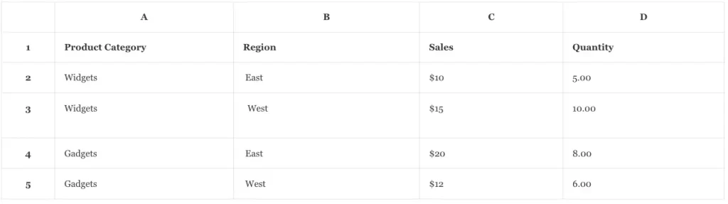
This dataset includes sales information for two product categories (Widgets and Gadgets) in two regions (East and West).
The Sales column represents the total sales for each product category in each region, and the Quantity column represents the total quantity of each product category sold in each region.

2.2.2 Add A Calculated Field To The PivotTable.

In this example, we will use the above dataset to create a PivotTable that shows total sales by region and product category.
Then add a calculated field to calculate the average selling price for each product category.
Before starting, make sure the Sales column cell value data type is Currency and the Quantity column cell value data type is Number.
And make sure there is no white space in the cell value’s beginning and end.
Now, create a PivotTable from the above data set, you can refer to the article How To Create, Remove Excel PivotTable Examples to learn how to do it.
Because we want to calculate the average selling price for each product category, we can create a calculated field with the following formula: =SUM(Sales)/SUM(Quantity). This formula divides the total sales by the total quantity to calculate the average selling price.
Select the PivotTable and click the “PivotTable Analyze” tab in the Excel ribbon.
Click the “Fields, Items & Sets” item in the Calculations group and select “Calculated Field” from the drop-down list.
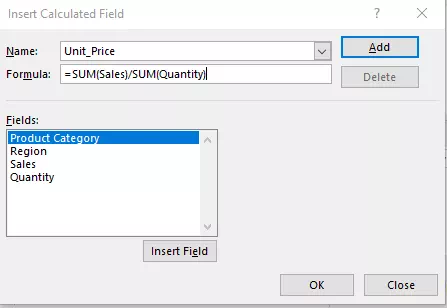
Input the field name Unit_Price in the Name text box, and input the formula =SUM(Sales)/SUM(Quantity) in the Formula input text box like below.
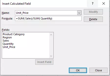
Click the Add button, then it will add the newly created calculated field ( Unit_Price ) in the Fields list.
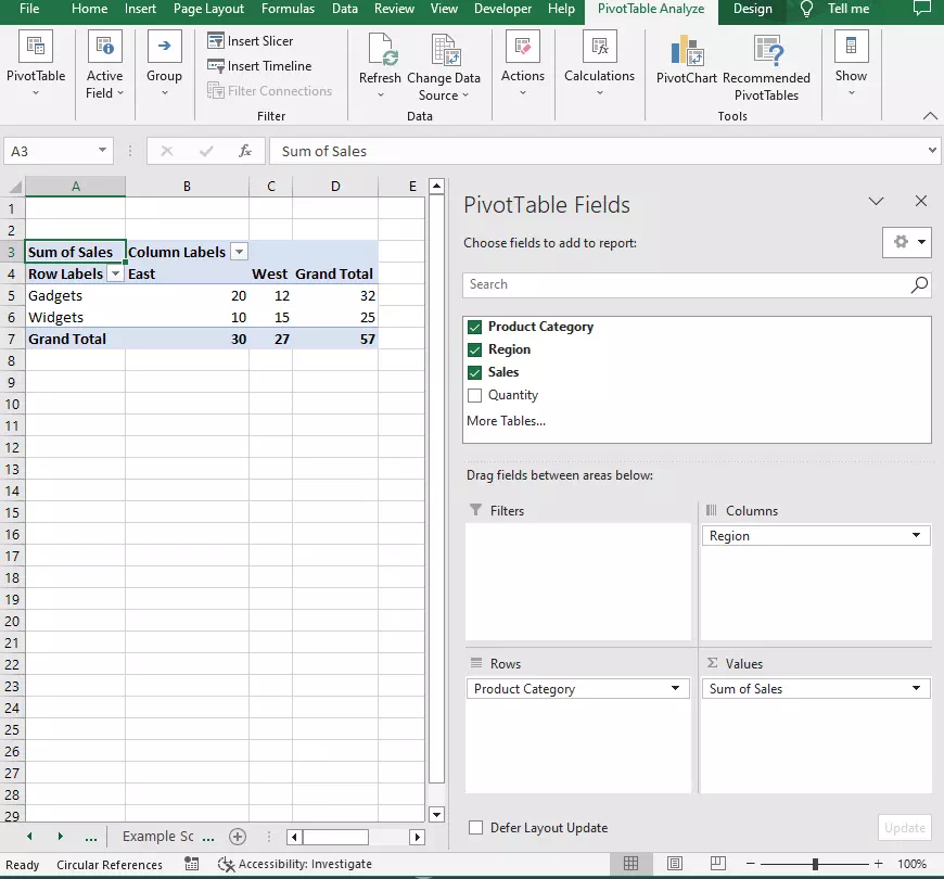
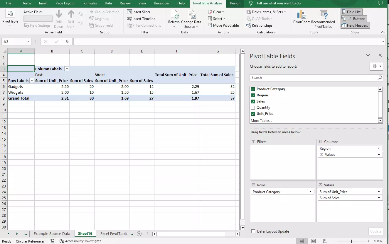
After you click the OK button, you can see the calculated field is added in the Excel PivotTable pane like below.
You can drag it to the Values column to show the calculated field values in the PivotTable as you need.

References

How To Modify, Delete Calculated Field In Excel PivotTable.