How To Use Excel Match Function With Examples

The excel MATCH function is used to find a value in a cell range, it will return the position number of the search value in the cell range. After that, we can use the Excel INDEX function and the position number to get the matched cell data. This article will tell you how to use the Excel INDEX MATCH function together with examples.

1. How To Use Excel Match Function.

1.1 Excel Match Function Syntax.

1. The Excel MATCH function has the below syntax.

   =MATCH(lookup_value, lookup_array, [match_type])

2. The first argument lookup_value is the keyword data (number or text) that will be searched in the second argument lookup_array.
3. The second argument lookup_array is an array or a cell range that will be searched in.
4. The third argument match_type is a number value.
5. When the number is 1 it means to look up the first maximum number in the lookup_array that is less than or equal to the lookup_value, this match type needs to sort the lookup_array in ascending order.
6. When the number is 0 it means to look up the first value in the lookup_array that is equal to the lookup_value exactly, this match type does not need to sort the order of the lookup_array elements.
7. When the number is –1 it means to look up the first minimum number in the lookup_array that is greater than or equal to the lookup_value, this match type needs to sort the lookup_array in descending order.
8. The MATCH function will return the position number of the first matched array element or cell in the lookup_array.

1.2 Excel Match Function Examples.

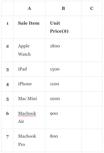
1. Below are the Excel match function example data cells.
   
2. Because we need to sort the above rows, so we need to convert the above cells to an Excel table.
3. You can read the article Excel Convert Table To Range Example And Vice Versa to learn how to convert cell range A1:B7 to an Excel table, below is the table after conversion.
   

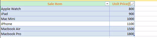
1.2.1 Excel Match Function Match Type Less Than Example.

1. Click the Down arrow on the right side of the cell Unit Price($) and sort column B in ascending order by selecting the Sort Smallest to Largest item.
2. Input the formula =MATCH(850, B2:B7, 1) in cell C2 and press the enter key, then it will display the number 1 in cell C2.
3. This is because only the first cell (containing the number 800 )’s value is the biggest number which is less than the lookup_value (850).

1.2.2 Excel Match Function Match Type Greater Than Example.

1. Click the Down arrow on the right side of the cell Unit Price($) and sort column B in descending order by selecting the Sort Largest to Smallest item.
2. Input the formula =MATCH(850, B2:B7, -1) in cell C3 and press the enter key, then it will display the number 5 in cell C3.
3. This is because the fifth position cell ( contains number 900 )’s value is the smallest number which is greater than the lookup_value (850).
4. And you can see that cell C2‘s value has been changed to #N/A, this is because cell C2 contains the formula =MATCH(850, B2:B7, 1) which sets the match_type value to 1 in the formula.
5. When you set the match_type value to 1, it needs to sort the lookup_array (cell range B2:B7) in ascending order.

1.2.3 Excel Match Function Match Type Exact Match Example.

1. Input the formula =MATCH(850, B2:B7, 0) in cell C4 and press the enter key, then it will display the error text #N/A in cell C4.
2. This is because you set the match_type argument to 0 which means the exact match and the cell range B2:B7 do not contain a number 850.
3. Change the formula to =MATCH(800, B2:B7, 0) and press the enter key, then it will display the number 6 ( the cell position in my example).
4. The exact match type does not need to sort the lookup_array.
5. You can use the wildcard in the exact match lookup_value, the character * will match multiple characters and the character ? will match a single character.
6. The formula =MATCH(“iPa?”, A2:A7, 0) will return the number 2 ( which cell value is iPad ).
7. The formula =MATCH(“*mac*”, A2:A7, 0) will return the number 4 ( which cell value is Mac Mini ).
8. Because the cell value Mac Mini is the first cell that contains the lookup_value *mac*.
9. And the MATCH function is case-insensitive.

2. How To Use Excel Index Match Function To Get The Matched Cell Value.

1. After you use the Excel MATCH function to get the lookup_value position in the lookup_array, you can use the Excel INDEX function to get the searched cell value.
2. Below is the example data table.
   
3. If we want to search the keyword mac in Sale Item column and return the first matched cell value, we can use the formula =INDEX(A2:A7, MATCH(“*mac*”, A2:A7, 0)).
4. The MATCH(“*mac*”, A2:A7, 0) function will return the first matched cell’s position in the cell range.
5. The INDEX function will return the cell value in the cell range using the above cell position value.