How To Use OFFSET Function In Excel

The excel OFFSET function can be used to get the reference to a cell or cell range from the starting point ( cell ). It is very useful when you use it correctly. This article will tell you how to use it with some examples.

1. Excel OFFSET Function Introduction.

1. The OFFSET function has the below syntax.

   OFFSET(reference, rows, cols, [height], [width])
   

2. The first argument reference is the starting cell address such as A1.
3. The second argument rows are the number of rows that offset from the starting cell.
4. If the rows argument is a positive number then it means to move down, if the rows argument is a negative number then it means to move up.
5. The third argument cols are the number of columns that offset from the starting cell.
6. If the cols argument is a positive number then it means to move to the right, if the cols argument is a negative number then it means to move to the left.
7. With the above 3 arguments, you can get the reference of the target cell range’s top-left cell.
8. The fourth argument height is the target returned cell range rows number if provided.
9. The fifth argument width is the target returned cell range columns number if provided.
10. The excel OFFSET function can only return the referenced cell range, it can not move the cells.
11. The first argument of the OFFSET function should be one cell or adjacent cells, if not the function will return the #VALUE! error text.
12. If the returned reference cell range is over the excel spreadsheet’s edge, you will get the #REF! error text.

2. How To Use Offset Function In Excel Example.

1. In the below table, if you want to get the reference to cell range C3:D4 from the starting cell A1, you can input the formula =OFFSET(A1,2,2,2,2) in any cell.
   
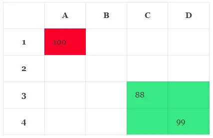
2. The rows and cols argument value can be a positive or a negative number.
3. When the rows and cols argument is a negative number, then it means offset to up rows and left columns from the starting cell.
4. For example, OFFSET(D3,-2,-3) will return the reference to cell A1.

3. How To Offset From The Current Active Cell.

1. You can use the formula =OFFSET(INDIRECT(ADDRESS(ROW(), COLUMN())),1,-1) to offset from the current active cell.
2. The ROW function returns the currently active cell row number.
3. The COLUMN function returns the currently active cell column number.
4. The ADDRESS(ROW(), COLUMN()) function returns the currently active cell address text.
5. The INDIRECT(ADDRESS(ROW(), COLUMN())) function returns the currently active cell object reference.
6. And finally, the =OFFSET(INDIRECT(ADDRESS(ROW(), COLUMN())),1,-1) formula can return the cell offset 1 row down and 1 column left to the currently active cell.