How To Sum Dynamic Range In Excel

The Excel SUM function can calculate the summary of number values in a cell range. But when you add a new number cell before or after the cell range, the SUM function can not add the dynamically added number in the result. This article will tell you how to sum dynamic range in Excel.

1. Sum Dynamic Range In Excel Example?

1. Below are the example data cells.
   
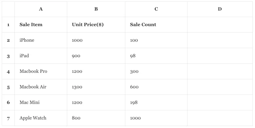
2. Now input the formula =SUM(C2:C7) in cell D1, then it will summarize the number values in the cell range C2:C7 and show it in cell D1.
3. But when you add a new row after row 7, the formula will not add the newly added cell (C8) number value.

2. Sum Dynamic Range In Excel Using Excel Table.

1. You can use the Excel table to fix the above issue.
2. Select the cell range A1:C7, then click the Excel Insert tab —> Table item in the Tables group to convert the cell range into an Excel table ( you can refer to the article Excel Convert Table To Range Example And Vice Versa ).
3. Click the Table Design tab on the Excel top menu bar, then you can change the Excel table name in the Properties group Table Name input text box.
4. In this example, I change the table name to Table_Sum.
5. Now input the formula =SUM(Table_Sum[Sale Count]) in cell D2 and press the enter key, then it will summarize all the cell number values in column C.
6. In this example the table name is Table_Sum and the column name is Sale Count.
7. Right-click one row in the table and click the menu item Insert to insert a new row ( the red row ) in the table like below.
   
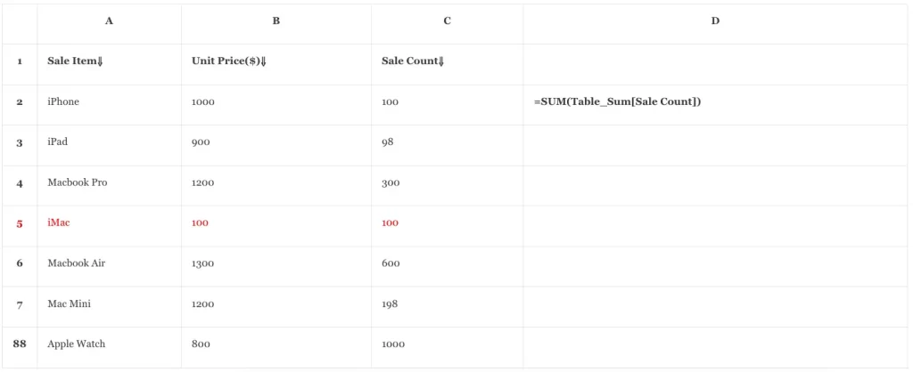
8. You will find that the summarized number value in cell D2 is changed automatically also, it includes the newly inserted row’s sale count number.

3. Sum Dynamic Range With Special Criteria In Excel Using INDEX & MATCH Function.

1. We can also use the Excel INDEX & MATCH function together to summarize the dynamic range number value in Excel.
2. Below are the example data cells, we add a Search Sale Count number in cell D1, and a Total Result Number in cell D4.
   
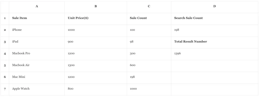
3. Input the formula =SUM(C2:INDEX(C2:C7, MATCH(D2, C2:C7,0))) in cell D4.
4. Now if you input a number such as 198 in cell D2, then it will show the number 1396 in cell D4.
5. The number 1396 is the summary of the number value in the cell range C2:C6 because cell C6 contains the number 198.
6. First, the function MATCH(D2, C2:C7,0) will return the cell index number 6 ( which matches the value in cell D2 exactly )in the cell range C2:C7.
7. Then the function INDEX(C2:C7, MATCH(D2, C2:C7,0)) will return the matched cell C6 from the cell range C2:C7.
8. Finally, the formula =SUM(C2:INDEX(C2:C7, MATCH(D2, C2:C7,0))) will summarize the number value in cell range C2:C6 and get the resulting number.
9. You can read the article How To Use Excel Match Function With Examples to learn more.

4. Sum Dynamic Range With Last None Empty Cell In Excel Using LOOKUP Function.

1. If you want to summarize the cell number until the last non-empty cell in a column, you can read this example.
2. You can first use the Excel LOOKUP function to find the last non-empty Excel cell in a column ( please refer to the article Excel Find First / Last Non-Empty Cell In Row / Column Example ).
3. Then use the MATCH function to get the last non-empty cell’s index number in the cell range.
4. Then use the INDEX function to get the last non-empty cell.
5. Then use the SUM function to summarize the column cell’s number values until the last non-empty cell.
6. In this example the LOOKUP function is LOOKUP(2,1/(NOT(ISBLANK(C2:C7))), C2:C7), it will find the last non-empty cell.
7. Then use the MATCH function to get the last non-empty cell’s index number in the cell range C2:C7, the function is MATCH(LOOKUP(2,1/(NOT(ISBLANK(C2:C7))), C2:C7), C2:C7,0).
8. Then use the INDEX function to get the last non-empty cell, the function is INDEX(C2:C7, MATCH(LOOKUP(2,1/(NOT(ISBLANK(C2:C7))), C2:C7), C2:C7,0)).
9. Finally, use the SUM function to summarize the column cell numbers from the first cell to the last non-empty cell, the formula is =SUM(C2:INDEX(C2:C7, MATCH(LOOKUP(2,1/(NOT(ISBLANK(C2:C7))), C2:C7), C2:C7,0))).